PART TWO of Sauron - Intelligent Marine surveillance system:

PART THREE

Getting started with Axelera Metis & Degirum

On boot up, first we need to make sure the Axelera Metis device is loaded properly and working using voyager-sdk. Open new terminal and refresh the Metis device as following:

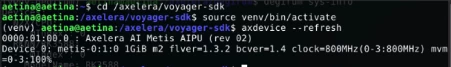
This should only be needed once after power up.

Before staring the Maritime Surveillance application, we need to make sure the Degirum sdk can see the Axelera device, and the appropriate virtual environment is loaded. In my case I installed the degirum tools in /axelera/degirum/ folder.

cd /axelera/degirum/
source venv-degirum/bin/activate
degirum sys-info

Device settings:

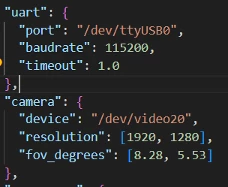
At this point we need to make sure we have the correct device settings in the settings.json file. Mainly we need to make sure we specify the correct device names for the USB3 camera as well as the serial port for communications with the STM32 controller.

To check which Serial port is the one:

ls /dev/tty*
dmesg | grep tty

In my case, I am using a CP210x based USB-UART device so I saw the following output, confirming the correct device to be ttyUSB0

[    3.136576] usb 3-1: cp210x converter now attached to ttyUSB0

For getting the device name for the USB3 camera, I use:

ls /dev/vid*

By repeating this command with camera unplugged and then plugged, you can infer the correct device name. Then update these in the settings.json file

Setting up scan zone

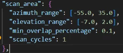
In very simple terms, the system lets the user define a “scanning zone” in terms of azimuth and elevation angle ranges in front of the gimbal. This is the area we want scanned continuously. In my case, I set it to the extents I could see on both sides. The angles are in gimbal coordinates, with zero azimuth angle in front of the gimbal.

Setting up restricted zones:

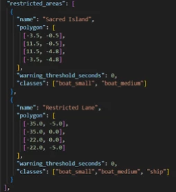
The user also defines “restricted zones” and rules for the restricted zones. All of these are defined in the settings.json file. User can specify these zones as non-self-intersecting, closed polygons and define alarm rules for each polygon. These rules state what classes of detected objects the rule applies to, and as how much dwell time to tolerate for the unauthorized classes of objects in that zone. User can define as many zones as desired and needed.

Since all these angles are in gimbal azimuth, elevation angles, I have provided a utility that lets the user easily find the angle coordinates for the scan range and zones.

Launch the application using the –live-video argument and press “I” to get angles of any point the crosshair is pointed at.

python main.py –live-video

To explain this, I have made a short video to demonstrate this:

Note that there was an issue with the audio recording in the last ~10 seconds. What I said at that time was that you can also use this –live-video mode to get your C mount camera to focus very accurately, which is very important to detect objects that are very far and small.

Operation of Maritime Surveillance System

In very simple terms, the operation is as following:

Once the user has defined the “scan zone” and one or more “restricted zones”, the user will then execute the main application with any arguments:

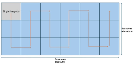
python main.py

The application will divide the scan zone into equally spaced image positions based on the camera FOV and a user-define minimum overlap percentage between adjacent positions. Then the program will arrange them into a serpentine motion plan starting from top-left (seeing from camera perspective) all the way to the right-end of the scan zone. I have made a diagram to explain this:

Then the application turns on the gimbal and feeds the position commands to the gimbal one by one. Once any image position is reached the gimbal confirms this by retrieving the gimbal position. Each location is re-tried up to 3 times (configurable in settings file) if needed. Once the gimbal position is confirmed, the application snaps a fresh image from the camera (making sure to discard any old images in the pipeline first) and sends this to the degirum pysdk’s tiling inference function. The pysdk chops the image into 6 times of 640x640 each and performs inference on each. It then does one inference on the full image resized to 640x640 also. Then it combines all results and maps them into the original image coordinates.

Once detection results are obtained, then the program tests each detection to check if it’s inside any of the restricted areas. If it is, then it will pull out past history to check if the time criteria is met (for example if a “boat_small” has been lingering in an area for more than the specified amount of time. If time threshold is specified as 0 in settings, it means as soon as an object of the specified classes is found inside a restricted area polygon, an alarm will be raised. The application raises this as an alarm on the screen in red, and also puts a red bounding box around the object raising alarm to make it visually clear. The application also include code for audible alarm over Bluetooth. However, I had some issues with my Bluetooth driver in the last few days and so I did not include it in the demo videos.

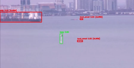
In the above image, you will notice that the ship and boats are marked in red but not the marine buoy. This is because in the “restricted area” settings for this particular area, we asked to trigger only for boats and ships. Of course we want this control so that fixed objects like marine buoys don’t trigger alarms even though we still want to monitor they are staying in their place for the safety of the ships.

Anyway, without further ado, here are a few videos from the runs I did with a voice over for more details.

For reference, here is an image of the sea being scanned from my cellphone camera at 1x. 

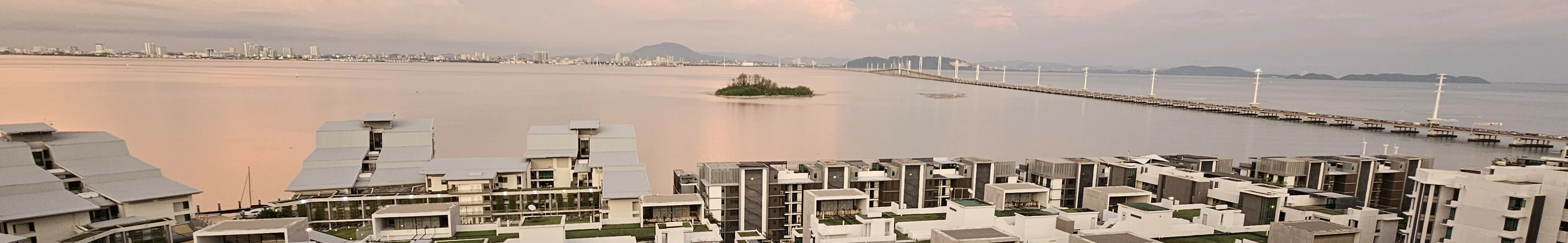
The amazing thing to note is how far a lot of the detected objects in the video are. Of course detecting a huge oil tanker at 5km is no big deal. But amazingly even the smallest fishing boats are being detected very reliably up to 10kms away!

Note that in these videos I run one scan cycle at a time. However, this is a configurable parameter inside the settings.json file (“scan_cycles”) and specifying -1 means continuous (infinite) monitoring.

Note that the application also logs all detections in a csv file with all the details. This file can later be potentially processed for more detailed insights into the marine activity. The annotated images are also saved for reference (filename for each detection is logged in the .csv file).

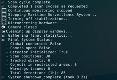
During the whole time the system is running, messages are logged to the console. At the end of the run, the system is properly shut down and a summary is presented to the user:

Other features:

Data collection feature:

After going through the pain of manual image collection for building dataset, I realized that the gimbal system is a great way to collect further data to refine the model. For example, previously I took most of my images in broad daylight and now I observe excellent results in daylight conditions, but as it starts to get dark, false positives start to increase. Adding images in low lighting is sure to improve model accuracy in dark conditions as well. Now I have an easy way to accomplish this.

See the relevant settings in settings.json:

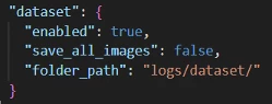
When enabled (default), depending on the value of “save_all_images”, the program will either save every acquired image to the dataset folder, or save only images with at least one detections. Both have their use case. Note that this can be extended to save images with annotations also. The reason I did not do it yet is because I wanted to first select a format that is most accepted before implementing it. This would save the annotating time when adding new images to dataset.

Future plans & potential for improvements:

Working on this project was a lot of fun and I learnt a lot of new things. Once the system got up and running, ideas started flowing to me on else can be done to extend the system’s functionality.

1. Currently objects are detected and logged in the (azimuth, elevation) coordinate system but it would be even nicer to map detection to a map, for example. Certain objects and features in images should stay fixed and it should be possible to either manually stake visual points to points on a map and then calculate a transform for this mapping. It may even be possible (and even better) to train a model that can, for example, find buoys on a google-earth map and then map buoy detections in the general vicinity to the positions on the map. Once this is done, it should also be possible to map other detections to positions on the map.
2. Implementing a re-id/tracking model to correspond detection of objects from one scan to another.
3. Extending the system to detect and track birds flying over the sea. I often see falcons flying over the sea and it would be nice to detect them and track them to study their behaviour.
4. Implement tracking algorithms: This is an easy one if done with opencv trackers. However, since the Metis device make such huge amount of processing power available, I am curious about converting one of the state-of-art deep-learning based visual tracking algorithms to Axelera and deploying to see how fast it can go. OpenCV trackers have limited performance and the better ones are too slow to run for some real time applications.

Final words:

I am very thankful to Axelera to provide me the opportunity to work on this project. I thoroughly enjoyed working on it and learnt so much. I also found the Axelera team to be very helpful during this whole process. I also want to thank the team at Degirum for their support, guidance and help in getting my project up and running. Working on this project has opened my eyes to new possibilities and I am excited about what I build next.

Link to Github project: https://github.com/SaadTiwana/axelera